Part 4: Going deeper with a counting problem
This project is about deep learning, but nothing has been remotely deep so far. The model discussed in the last part was so shallow that it could have easily been trained by hand!
In this post, we will explore the possibility of training a deeper neural network, one in which we will give up control and let the data speak for itself. Not only that, but we will also address a more complicated problem: counting how many moves are possible on a given grid.
A deeper neural network
Let us begin with the network. Instead of having one convolutional layer with a big kernel doing all the work, we slice our model into several layers. The advantage of doing so is that each individual layer need not be as complicated.
Our first layer will be a convolutional layer with a 3 x 3 kernel and stride 3: its role is to break down the grid into blocks of 3 x 3 pixels, each corresponding to a point (the pixel at the center) and 8 segments attached to it (one in each direction).
After that, we add four more convolutional layer with kernel size 2 x 2. Their role is to examine the relations between nearest neighbors. The input of the first of these layers is a block of 3 x 3 pixels; its ouputs have a receiptive field of 2 x 2 blocks, or 6 x 6 pixels. After 4 layers, the receptive field is 5 x 5 blocks, or 15 x 15 pixels. This is sufficient to detect the relevant features that are spreading over 13 x 13 pixels at most.
To keep track of sufficiently many possible combinations of neighboring blocks, we use 40 channels in each layer (a bit less in the first layer). This number is motivated by the fact that there are eventually 5 combinations of lines and dots in 4 directions that give a possible move, and therefore 20 different features to discover. Using twice as many channel should be sufficient to do so.
The rest of the network consists of a pooling layer, followed by a couple of linear layers to turn the output into a single number. As a warm-up, we train the network on the same problem as last time. For this we use max pooling and two linear layers only.
In summary, the network architecture is the following:
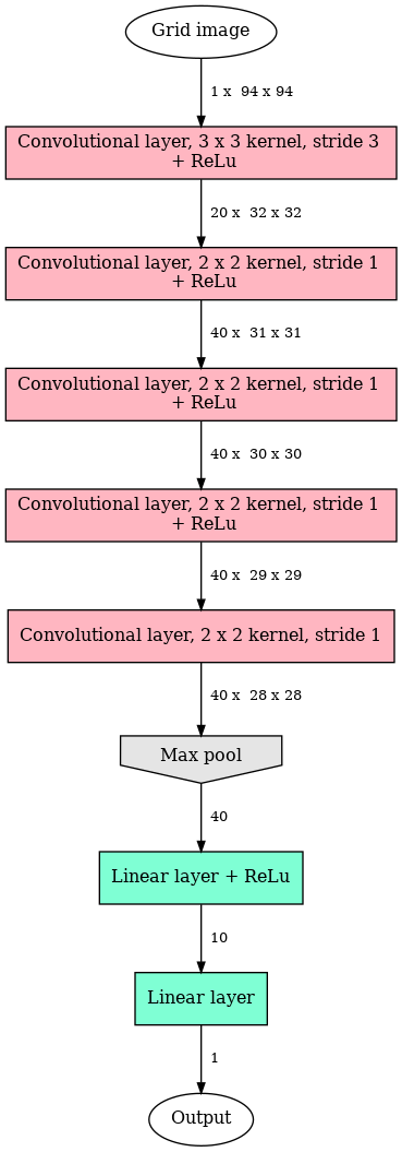
This model has 23,801 trainable parameters. This more than three times as many as our last model!
Training on the binary problem
The larger number of parameters together with the new depth of this network increases the risk of overfitting the data. Indeed, if we use a static set of 20,000 grids as we did last time, the network easily reaches 100% accuracy on the training set, while saturating at around 90% accuracy on a distinct validation set. We shall therefore use a dynamic data set, as discussed in Part 2: each grid is used 16 times for training (twice in each orientation), then discarded and replaced by a new one, generated on the spot.
More epochs are needed to train the model, but the process is more stable and we can therefore use twice the learning rate, namely 0.01. With these parameters the model is doing great! Here is how the accuracy evolves over 200 epochs:
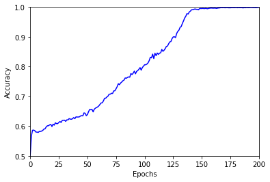
The final accuracy is 99.9%, above any reasonable expectation.
Counting: a more difficult problem
We are now ready to tackle a more difficult problem: we would like a model that counts how many possible moves there are in any given grid. The number of distinct possible moves is 28 at the beginning of the game (the empty grid with a cross pattern), and it is obviously zero when the game is over. In between, it varies a lot, and it is not uncommon to encounter grids with more than 30 different possible moves.
This is where all the difficulty of this new problem resides: the model must be able to discriminate between many possible outcomes. Our first problem was a classification problem (even though we used mean square loss from the start), whereas this is now a regression problem: the output of the network will be a number between 0 and 1 that is directly related to the number of possible moves (see below).
The different nature of the task also implies that we must use a slightly different model: our previous model was designed to identify at least one occurence of some feature; this new model must be able to count the relevant features. In practice, this means that we have to replace the max pooling layer by an average pooling layer. As the regression problem is more complicated, we will also add another linear layer before the finaly output.
In summary, the model architecture is made of the same convolutional layers as above, followed by this structure:
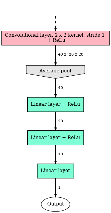
Note that we have also included a rectified linear unit (ReLu) before the average pooling layer to add a non-linearity there.
It turns out that training this model is difficult. So difficult in fact that it even fails at solving the simpler binary classification problem. But this is where transfer learning is going to help us. Instead of initializing the layers at random, we can use the values obtained earlier. Since both the model and the problem are new, we do this in two stages:
- In the first step, we train the new model on the old problem, starting with pre-trained convolutional layers (they share the same architecture) and randomly-initialized linear layers. This is done precisely as before, except from the fact that we use twice the learning rate (0.02) as most of the parameters are readily trained. The outcome of this procedure is summarized in this figure:
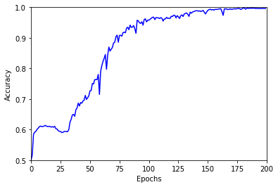
After around 30 epochs of stagnation, the accuracy increases steadily all the way to 99.5%. This is quite a laborious learning curve, given that most of the model was actually pre-trained, but the objective is attained: our new model with an average pooling layer gives an acceptable answer.
- In the second step we train the very same model on the new problem. Before reporting on the result, I need to give you a little bit more information on how the data is prepared and labelled.
New data
We want to create some grids and associate to each of them a label corresponding to the number of possible moves. This is easy to do with my Python implementation of the game in which the list of all possible moves is always available at every stage. The only tricky point is how do we generate a nice and uniform distribution of labels.
It turns out that a simple way of getting a pretty good distribution is to play a game at random until the end, then return to an arbitrary intermediate point chosen with uniform probability. This is the distribution of labels that we get in this way after playing 20,000 games:
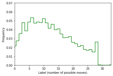
Okay, let’s be honest: this is far from being perfectly uniform. But all labels between 0 and 28 have a significant probability of being realized, and that is just what we need. Final configurations with no possible moves are slightly under-represented, but this won’t be a problem since we are working with a model that is already pre-trained to detect this special case.
The next step is to turn this label (a positive integer , let’s call it $n$,) into a real number $y$ that can more easily be fitted with the model. We will use
\[y = \frac{n}{n + 5}\]$y$ is now in the interval $[0, 1]$: it is zero if there are no possible moves $(n = 0)$, and it approaches 1 if there are many of them $(n \to \infty)$. This choice gives a mean value $\mu(y) \approx 0.6$, and a standard deviation $\sigma(y) \approx 0.2$. The variable $y$ is the value that the network will try to match. From its output $y’$, we recover the estimated number of possible moves $n’$ using the inverse relation
\[n' = \frac{5 y'}{1 - y'}\]The result
The training process is setup to minimize a loss function corresponding to the mean square error between $n$ (the label) and $n’$ (the prediction). However, to avoid dealing with singular values of $n’$ when the output is close to $y’ = 1$, we use instead the following function, which is regular everywhere in $y’$:
\[L(y, y') = \left( \frac{y - y'}{1 - y} \right)^2\]The accuracy of the model is measured comparing $n$ and $n’$. The following figure shows the evolution of the error rate over 500 epochs of training (one epoch corresponds to 100 mini-batches of 200 grids each).
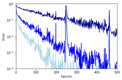
The darker line is the exact error rate (how often $n’ \neq n$), and the lighter lines the error rate with a tolerance of $\pm 1$ (how often $\left| n’ - n \right| > 1$) and $\pm 2$ (lightest line). As you can see, all errors are nicely decreasing as the training advances. After 100 epochs the network already predicts the right number with $\pm 2$ tolerance with 0.1% error. 300 epochs are needed to reach the same accuracy with $\pm 1$ tolerance. Finally, after 500 epochs the network makes an exact prediction more than 98% of the time, and when it fails it is always by at most one move.
It looks like the training could be pushed even further, but I decided to stop here. This is already quite a remarkable result!
Inference
Using dynamical data that is permanently generated as the training goes should prevent overfitting. But there are only a finite number of possible game outcomes, so how can I be certain that the model is really answering the question properly?
Well, one way of testing this is to expose the network to grids that it has never seen before. There exists a variant of the game of Morpion Solitaire in which the starting configuration is not a cross, but instead a “pipe”:
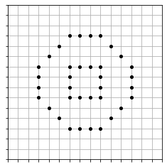
There are 24 possible moves in this configuration. The models’ prediction in this case is 23.89. That’s spot on! Playing a number of games starting with this configuration, I could verify that the model works indeed (nearly) perfectly.
Looking forward
Of course, the problem addressed here does not require deep learning: counting the number of possible moves for a given configuration is something that can easily be done in an algorithmic way. The neural network is nice as it can compute this number for many grids at once, hence slightly accelerating the process: it will in fact be used in the next post to try and improve our initial random exploration algorithm. But the two important goals that have been achieved are different:
- This is a proof of principle: I was able to define a relatively deep model and train it to solve a regression problem that is not so simple. All ingredients needed for tackling the real problem are essentially present here.
- This is also a valuable model to be later used in a transfer learning process. As we saw, this is key for making real progress.