Part 5: Playing with a model
I have been explaining so far how to use a deep neural network to describe data gathered from the game of morpion solitaire. Now it is time to use the neural network to improve the way the computer plays.
Choosing the right move
At any given stage of the game, a player of morpion solitaire is faced with the dilemma of choosing the next move among several options. Sometimes the decision is easy to make. For instance, this is a configuration that you may have reached after 20 moves:
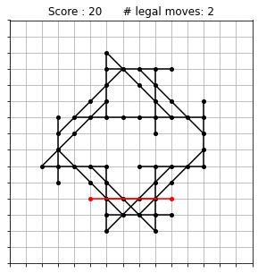
There are only two options left at this stage, shown here in red (the red lines are partly overlapping). The outcome of playing one or the other could hardly be more different. If you pick the point to the left, then the game is immediately over: there are no more possible moves and your final score is 21. If on the contrary you pick the point to the right, then you have the choice between two more moves at the next stage, and both of these moves open up a wealth of possibilities. This is a possible completion of the very same game, showing that it can go on for quite a while:
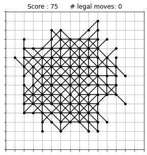
Clearly, choosing a move at random as we did in Part 1 is sometimes very dumb. If we can look ahead just one move, we can easily avoid this kind of bottleneck situations.
The model that I trained in the last part does not make very advanced predictions, but it just right to address this problem: given a list of possible moves, we can construct all corresponding grids and feed their images to the neural network. The outcome is a number that tells us whether more moves will be possible or not. This procedure is not only useful when there are a few moves left, but it is also good to assess whether a move opens up more possibilities or if it doesn’t. Choosing only the better moves will certainly give us better scores, right?
Weighted probabilities
However, we have to be careful not to remove all randomness in our computer exploration of the game. Who said that the world record is obtained making only optimal moves at each stage? Maybe it is sometimes good to make a move that will only prove useful after many more steps?
What we want is a weighted probability distribution: the computer will still choose the next move at random, but moves that generate more moves will be more likely. One way to implement this mathematically is as follows. Let’s say that our favorite neural network sees $n_i$ possible moves at next stage if we pick the move $i$ right now. Then we associate with move $i$ a probability $p_i$ defined by
\[p_i = \frac{\exp(\beta n_i)}{\sum_j \exp(\beta n_j)}\]$\beta$ is a parameter that we can choose freely. It is in some sense analogous to the $\beta$ denoting inverse temperature in statistical physics:
- When $\beta = 0$ (infinite temperature), then all probabilities are equal and we are back to choosing a move at random.
- When $\beta$ is a large number (low temperature), then the probability of choosing the move with the highest $n_i$ approaches one, and so the exploration is “frozen” in the situation determined by the “optimal” move at each stage.
Neither of these situations is good. We want to use some intermediate value for $\beta$. But which one? The best way to answer this question is to perform a little experiment. Let us play 1000 games in which we choose all moves according to this weighted probability distribution, and repeat the procedure with different values of $\beta$. In each case, we look at how many high scores we get. By this I mean scores that are higher than most results obtained in the random exploration. Let us place the threshold at 70. Here is what we get:
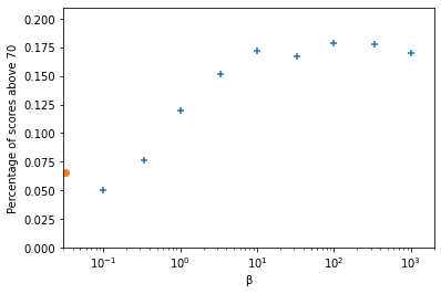
The orange dot on the left is the percentage of high scores that we found in the purely random exploration of the game ($\beta = 0$), corresponding to the distribution found in Part 1. The other data points are the result of our experiment. You can see that the percentage of scores at 70 and above climbs to nearly 20% when $\beta \gtrsim 10$, and that it is more or less stable above this value.
A specificity of our model is that there are often many moves with the same $n_i$, so even at very large $\beta$ there is a lot of randomness leftover. But since we don’t want a too large $\beta$ in principle, I am going to choose as my preferred value the beginning of the plateau, namely
\[\beta = 10\]The outcome
From now on we stick to this value and let the computer play 10,000 games using the model. This is how the new distribution of scores compares to the random exploration:
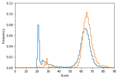
The new distribution is not fundamentally different, but:
- We nearly got rid of the very low-score games (less than 50).
- The main peak moved a little bit to the right, meaning that the final scores improved on average.
- The high-score tail to the right of the graph appears to be significantly thicker than before.
Let us zoom in on that last region:
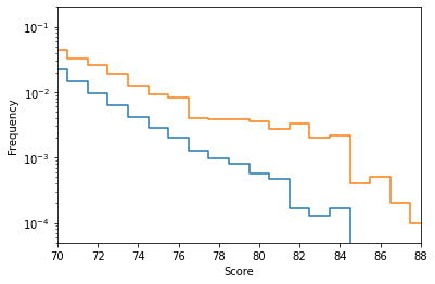
The frequency of high-score grids has doubled (or even more) over all of the range plotted here. It still takes about 1000 games to get once above a score of 85 on average, but the improvement is clearly visible.
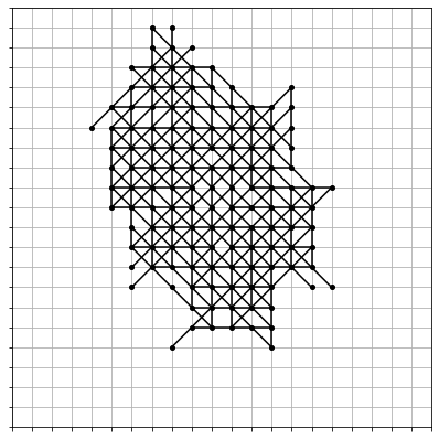
And as we could have expected, we found a new highest score in this exploration phase. Here is the new record grid, at an amazing 96 points:
Conclusions
We are still quite far from the world record, aren’t we? Even far from my own attempts by hand.
But this should not be a disappointment. The model used so far only looks one move ahead, and not more. Training a better model that can actually make predictions a few moves ahead is the goal of the next part. For now, it is great to see that all the different pieces come nicely together and already give a first improvement over our initial exploration.