Part 3: A simple binary problem
Now that we understand the dynamics of the game and we know how to generate large amounts of data, we are ready to train our first model. To begin with, we will focus on a simple problem: determining whether a grid is complete or not, meaning whether one can find at least one allowed move.
This sounds like a dumb problem to solve, and indeed it is: the information whether the game is over or not is already contained in its Python implementation. But we will pretend not to know and try to answer the question just looking at an image of the grid. Of course it is also very easy to write a simple loop that runs over all lattice sites and checks whether there is an allowed move there. But this is not what we want to do. We want to train a neural network without having to tell it how to do it. The input will simply be a large number of grids with labels indicating whether the game is over or not, and the net will learn the rules of the game by itself.
And even though the problem is a dumb one, it is quite instructive as a starter. In fact, when you think about it, this is not so much a simple problem even for a human: when you play the game with pen and paper and end up with a grid that has lots of points and lines, it takes time to verify that you are not missing one move. Let us see if the neural net can do this better.
The network
As this is a very simple problem, the neural net does not need to be very deep. In fact, a single convolutional layer can do most of the work.
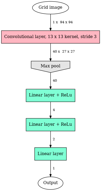
The drawback is that the convolutional kernel must be large enough so that a complete segment of 5 points and 4 lines can fit into its receptive field. In terms of the representation discussed in Part 2, this corresponds to a kernel size of 13 x 13 pixels. The first layer of the network will therefore be a convolutional layer with a 13 x 13 kernel, stride 3, and no padding, followed by max pooling. The goal of this layer will be to discover features corresponding to allowed moves in the vertical, horizontal, and both diagonal directions. While in principle only 4 channels are sufficient to do so, in practice these features have a lot of non-trivial structure that are not easy to detect in a stochastic process. We will therefore use many more output channels. Empirical testing shows that 40 is a good number: with less channels, the training tends to converge to a state in which only some of the features are detected (for instance it misses allowed moves in one of the directions).
Past this layer, the rest of the neural network only needs to implement a logic OR gate: if any allowed move is detected by the convolutional layer, the final answer is a yes; if no allowed move is detected, the final answer is a no. Few linear layers and channels are sufficient to do so. After some experimentation, we find that the following network architecture is fine for our problem:

This is one convolutional layer followed by 3 linear layers, with non-linearities given by max pooling after the first and rectified linear units (ReLu) between subsequent layers. The dimension of each layer’s input and output is indicated on to the arrows. Note that the large number of channels after the first layer (40) is immediately taken down to a very small number in the linear layers (4 channels and less).
This model has 6977 trainable parameters, most of which (6800) are inside the first layer. This is quite a large number for such a small network, and therefore a lot of data is required for training.
The data
For this problem, we make use of a static data set, in which all grids and labels are computed before the training begins. As we shall see in a minute, this is sufficient to achieve very high accuracy. Experimenting with dynamical data did not show significant improvement.
We let the computer play 10,000 random games. In each case, we keep an image of the final grid (with no allowed moves), and one image of an intermediate grid (with at least one allowed move). In this way the data consists in 20,000 grids, and it is perfectly balanced: 10,000 grids are given the label “0”, the other 10,000 the label “1”. The intermediate stage of the game is chosen at random in 1/3 of the games, with uniform probability distribution. In the other 2/3 of the games, we use the next-to-last stage, just before the last move is played: in this way most of the grids labelled with “1” have just one allowed move. If we do not use this trick, the neural net very quickly settles in a state in which it only verifies the presence of allowed moves in some of the directions, but not all 4 directions: this gives quite high accuracy for most of the games that have plenty of allowed moves, but it does not properly solve the problem.
Training and validation
The training follows a standard stochastic gradient descent (SGD) procedure. We use the PyTorch optimizer, with learning rate 0.005 and momentum 0.9. Stochasticity is introduced in the learning process through the splitting of data into 100 mini-batches of 200 grids each. Each time a mini-batch is fed to the network, we apply a transformation (90 degrees rotation or mirror flip), hence artificially augmenting the size of the data. In this way the neural net only sees the same data again after 8 epochs (an epoch corresponds to 100 mini-batches, or all of the data passing through the net). We use the mean square error as a loss function, keeping in mind that we eventually want to solve a regression problem.
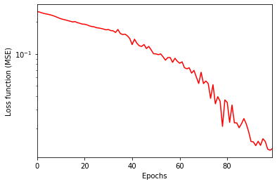
This is the behavior of the loss function over 100 epochs of training:

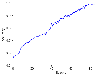
The loss decreases steadily, and the decay is even faster towards the end of the training cycle. I could have pushed the fitting procedure a bit further, but looking at the accuracy shows that a plateau has been reached after about 80 epochs:

The final value of the accuracy is 99%. It looks like the neural net has learned to answer the question. Yay!
How did it work?
Of course in this simple case my interest is not so much in the outcome of the training as it is in the process itself. What I am trying to do here is to understand how the network learns.
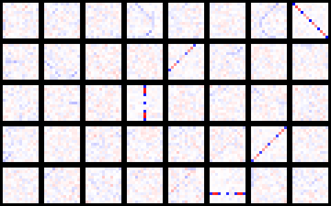
The shallow net used here is perfect to satisfy my curiosity: since nearly all the magic happens in the first layer, let’s take a look at its state after the learning process. Below is a picture of the convolution kernel in all 40 output channels. Each image has a size of 13 x 13 pixels, corresponding to the kernel size. Positive values are shown in blue (the darker the closer to +1), and negative in red (the darker the closer to -1). White pixels indicate kernel values close to zero.

The first observation is that most of the 40 channels are essentially zero: there are only significant features in 5 channels. Four of these features are obviously testing for the presence of allowed moves in each direction (horizontal, vertical, and both diagonals), whereas the fifth one (the incomplete diagonal in the second row) looks like an abandoned relic of the learning process .
It is also interesting to understand how the testing happens. For this, let us look zoom in on the channel in the third row, fourth column, which looks like this:

In this kernel the middle column has values close to +1 at the position of grid points (the 5 blue pixels) and -1 at the position of two segments (the 4 red pixels). All others entries are near zero. When this column is superimposed with an allowed move of the grid, the output is +4. In nearly all other cases, the output takes a lower value. For instance if any vertical segment is occupied, then at least one of the two segments at either extremity and contributes -2 to the sum. (Note that this strategy is used for the vertical and horizontal moves only; for both diagonal moves all 4 segments contribute negatively to the sum.) The logic implemented by the rest of the network is then clear: if the output (minus the bias) after max pooling is +4, then an allowed move has been found.
There is however a gap in the logic, and you will certainly have noticed it: if all 5 points are occupied, but none of the 4 segments is, the output of the convolution is +5, which is higher than the previous value and therefore picked up by max pooling. So how does the network react in this case? It turns out that the network incorrectly identifies an allowed move. After inspection, the remaining 1% of mistakes made by the network is all of this type: these are complete grids with no allowed moves, but in which there is a sequence of 5 points without segments in between.
Conclusions
So what should I conclude? Did the network fail to solve the problem? Maybe the result isn’t perfect, but I am definitely satisfied.
On the one hand the situation in which the network gives a wrong answer is rare enough. This is a binary classification problem, which means that whenever the network is wrong, it is completely wrong. But the broader goal of this project is to develop a network that gives a satisfactory estimation of a grid’s potential. The more precise the better, but if the network ends up being wrong by just one move every 100 predictions, the goal would certainly be attained.
On the other hand, it is also clear that better performances could be obtained with a deeper network. With a single convolutional layer followed by max pooling, obtaining a 100% perfect answer would require to combine different channels in a very non-trivial way, whereas the current training process found a simple alternative in which a single channel detects the presence or absence of an allowed move with 99% accuracy. Adding just one another layer before max pooling would for instance be sufficient to discriminate between the distinct outputs of the first layer (+4 vs. +5 in the case discussed above).
In the next part, we will precisely consider such a deeper network and try to answer a slightly more complicated question, before we dive into the core of the problem.