Part 2: The data

The goal of my project is to train a neural network to play morpion solitaire by itself. For this, a lot of data is needed. This piece describes how the data is gathered, how it is organized, and how it will later be fed into the neural network.

Game implementation

In the first part, I told you about the game. I showed some statistics and a few pretty pictures of different stages of the game. All of these were obtained from my own implementation of the game that you can find in my GitHub repository. The Python package MorpionSolitaire.py contains a few classes that let you play the game either following a random sequence of moves, using a model (this is what we want to develop), or manually step-by-step. It also provides simple methods to visualize the result in pictures. A Jupyter notebook with the package documentation is available in the same repository.

The Python object corresponding to a game of morpion solitaire (either a finished game or an on-going one) contains information about the game process: what succession of moves was used to get there, what are the allowed moves to do next, and so on. But this type of information will not be fed to the neural network. Our logic is to give as a sole input a snapshot of the grid, exactly as you would do with a human friend who is expert at the game: you show them the grid, and they tell you how many more moves you can hope to make if you play well.

The grid

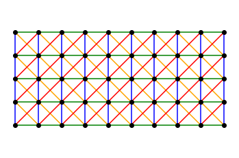
The grid is a 2-dimensional lattice, which for simplicity we will take to have fixed dimensions 32 x 32. This is sufficiently large to fit in the world-record grid, and yet sufficiently small to be easily processed by the neural network. Each lattice site has 5 boolean variables, describing the presence of a point, of vertical, horizontal or diagonal lines. If we distinguish these 5 variables with different colors, a piece of the lattice would look like this:

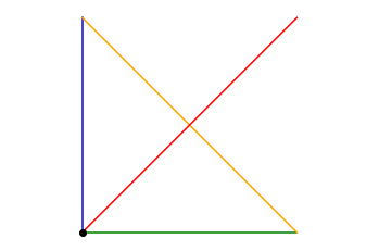
In total, there are 32 x 32 = 1024 unit cells that each look like this:

This is how the grid is coded in my Python implementation. In machine learning language, it can be viewed as a 5-channel image of size 32 x 32. But this way of encoding the data is a bit annoying. For instance, the image cannot be easily rotated by 90 degrees: after rotating all five layers, one needs to shift some of the layers to make sure that a line connecting two points still connects the same pair of points. In other words, this representation does not take into account the fact that the lines sit between the points.

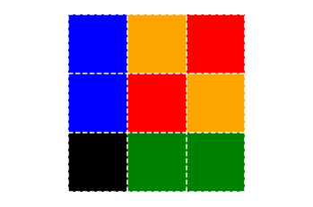
For this and other reasons, I find it more convenient to describe the grid as a single-channel image in which each unit cell is represented by 3 x 3 = 9 pixels, as follows:

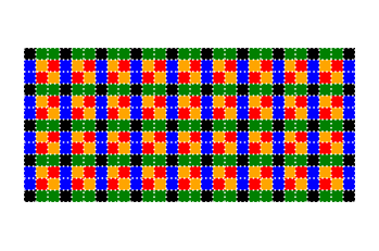
Note that the colors are matching: the vertical blue line above is replaced here by two blue pixels, and so on so forth. When the cells are put next to each other again, the piece of grid shown above now looks like this:

This representation is obviously redundant: it uses 9 bits of data where there were originally 5 bits. But this is still not so bad in terms of volume: each grid is now a single-channel black-and-white 94 x 94 pixel image (this is 2 pixels short of 3 x 32 = 96: I crop the edge of the lattice so that its boundary is made of points, vertical and horizontal lines, just like in the image above).

As an example, this is a series of 5 images corresponding to intermediate steps for one of the games described in part 1:

This representation is not only nice for humans (a glance at the image gives you a good impression of the game), but it is also very convenient in the learning process: it is well-suited to perform simple transformations for data augmentation, such as rotations by 90, 180 or 270 degrees, and horizontal or vertical mirror flip. This gives an effortless way of feeding “new” input to the neural network.

Also very importantly, this representation is model-independent: if I were to use 5-channel images in the deep learning process, then I would have to remember very precisely which channel encodes what data about the game, and this is dependent of the implementation. Instead, there is a unique way of encoding the grid in a single-channel image. So if you decide to start your own project of deep learning Morpion Solitaire, we can directly compare our models!

The neural network

It is too early to precisely define the model architecture that we will use at this stage. This architecture will depend on the exact problem that we want to solve, and we will only gradually increase the complexity of the task, starting with a simple problem in Part 3.

However, some general features of the neural network are already dictated by properties of the data:

• The outcome should not depend on the position of the grid in the image. If all points and lines are shifted by one unit to the left, the neural network should not see the difference. For this reason, the first layers of the neural net will be convolutional ones, followed by max/average pooling.

• Even though all images are for now of identical size, one can imagine cropping them (there is a lot of empty space around) or instead increasing their size should we obtain large scores. This speaks in favor of max pooling instead of averaging, as this is automatically independent of the image size. On the other hand, we might sometimes need to count how many features we find, and average pooling is better suited to do so. We will therefore use both methods depending on the context.

• Not all pixels in the image carry the same type of information: some represent points, other lines of the original grid. To preserve this information, the first convolutional layer should have stride 3 (or a multiple of 3) and no padding.

Therefore the typical structure of the neural net will be the following:

1. A convolutional layer with stride 3. The size of the kernel might vary.

2. Some more convolutional layers with stride one: this is where the relationship between neighboring sites of the grid is established. Most of computational power of the network happens in these layers, so the more the better. With deeper networks, skip connections might be needed to improve the learning abilities of the model, as in residual networks (ResNets).

3. Max pooling and flattening of the image.

4. A few linear layers to transform the output of the convolutional network into a simple result, typically a single number.

Data generation

Finally, the data is not worth anything without proper labelling. As with the network, the details of this procedure are quite dependent on the precise problem, and therefore most of it will be discussed later. Nevertheless, let me emphasize that this part of the problem is very time-consuming: the focus of my Python implementation of the game is on modularity, not performance, and as a consequence playing the game and exploring different possible outcomes takes time.

Two opposite approaches can be used to generate the data:

• A static approach in which a large data set with labels is created once and for all, and the model training takes place afterwards. The obvious risk with this approach is to overfit the data.

• A dynamic approach in which each piece of data used to train the network is created as needed. This completely removes the risk of overfitting, but it massively slows down the learning process.

In most cases, I will make use of an third, intermediate option:

• A hybrid approach in which each grid (or rather each mini-batch) is used multiple times but thrown away after a while. This prevents overfitting, and at the same it reduces the computer resources compared with the purely dynamical approach. It is also nicely compatible with the data augmentation mentioned before: each single grid can be used in 8 different orientations (4 rotations and one mirror symmetry).

This concludes what can be said about the data without entering the details of a particular problem. In the next part, I will describe a basic problem in which a neural network is trained to answer a simple yes-or-no question about the grid.